On this website I will try to guide you through the interactive part of the practical DFT lecture. Hopefully this will be interesting and useful for you!
We will be using the Atomic Simulation Environment (ASE) in conjunction with the DFT code GPAW.
Google Colab
Both ASE and GPAW operate through Python. We will be using Google’s Colab service to make it easy to follow along. No need to install Python
locally - you only need a browser. Our code will be running in a Jupyter notebook using Google’s resources.
To access a Python notebook just follow this link and
then click on ‘File’ > ‘Save a copy in Drive…’
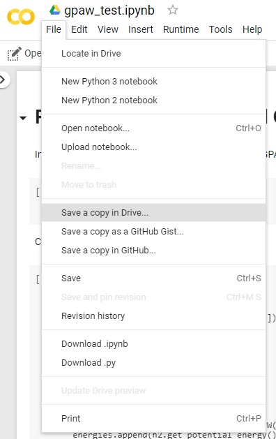
Once you have copied the notebook to your Google Drive you can edit, execute and work on it.
1. ASE Basics
Importing modules
First, we need to install ASE and GPAW on the server (%%capture represses output of the notebook cell). This installation works again (as of 6/5/2023) thanks to a question answered on StackExchange (credit goes to mazay0 and jboy).
%%capture
!apt install python3-mpi4py cython3 libxc-dev gpaw-data
!pip -q install gpaw
Then we can import the necessary packages into the Python notebook
from ase import Atoms  # The Atoms object is used to define and work with atomic structure in ASE
from ase.io import read, write  # The ase.io module is used to read and write crystal/molecular structure files
from gpaw import GPAW, PW  # GPAW will be our main DFT calculator and PW is the plane wave mode
This has typically one of the following forms (if .module is specified only a specific module of a Python package is imported, otherwise the whole package is considered):
import package.module as pm  # let's you access functions/objects like so: pm.function
from package.module import function  # imports object or function from package.module
from package.module import *  # imports all functions/objects
import package.module  # same
This is sorted from best to worst practice when it comes to importing modules in Python.
Creating our first atomic structure
First, let’s create a H2 molecule (experimental distance is 0.74 Angstroms) and add some vacuum padding around it
h2 = Atoms('H2', [(0, 0, 0), (0, 0, 0.74)])
h2.center(vacuum=2.5)
To export the atomic structure we created we can use the ase.io module
write('h2.cif', h2)
and we can let ASE tell us the cell parameters and atomic positions of the object we created
print(h2.cell)
print(h2.positions)
For a full list of atomic properties we can set and access refer to this link.
Set GPAW calculator
Now, let’s define a calculator using GPAW. We are specifying the exchange-correlation functional, k-points, the plane wave energy cutoff and a file to safe the calculation results.
calc = GPAW(xc='LDA',
            kpts=(1,1,1),
            mode=PW(500),
            txt='h2.txt')
Then we need to “attach” our calculator to the H2 molecule we created earlier.
h2.set_calculator(calc)
Evaluate properties
Using the calculator (GPAW) we now can simply calculate the energy of the atomic object and could either directly return it with print
or safe the result in a variable (e.g. result)
print(h2.get_potential_energy())  # or
result = h2.get_potential_energy()
Alternatively, we could also get the forces by .get_forces() among many other things.
Testing for convergence
Python’s for-loop greatly facilitates the testing for convergence (without tediously rewriting input files and continuously reading out energy results)
cutoffs = [100,200,300,400,500,1000]
energies = []

for cutoff in cutoffs:
  calc = GPAW(xc='LDA',
              kpts=(1,1,1),
              mode=PW(cutoff),
              txt='h2.txt')
  h2.set_calculator(calc)
  energies.append(h2.get_potential_energy())
print(energies)  # eV
here cutoffs is a list of energy cutoffs and the for-loop iterates over each entry and then adds the calculated energy to the (at first empty) energies list.
Displaying results and analysis
Now we can plot the results with matplotlib and by taking use of the time package we can get a little bit insight on how long the calculations
are taking when we increase the energy cutoff.
Further, we can get the electron density by calc.get_all_electron_density(), then sum over the x-direction and plot a 2D contour plot.
2. Atomization energy of H2
Let us look at one more example: By calculating the energy of diatomic hydrogen and the energy of mono-atomic hydrogen we can get the atomization
energy (or bond energy) given by \(2\cdot E_\mathrm{H}-E_{\mathrm{H}_2}\).
Link to the notebook can be found here.
How do LDA and PBE compare to the experimental value?
3. Elemental transition metal crystals
The structures of pure/elemental (transition) metal crystals are easy to describe because the atoms that form these metals can be thought of as identical perfect spheres.
The same can be said about the structure of the rare gases at very low temperatures. These substances crystallize in one of four basic structures that arise
from closely packing spheres:
Simple cubic (SC), body-centered cubic (BCC), hexagonal closest-packed (HCP), and face-centered cubic (FCC, sometimes called cubic closest-packed or CCP).
For this interactive part, each person should pick a transition metal from this list.
Write your name next to one element to claim it.
Creating the crystal and convergence tests
Open the next notebook here.
The ase.build module comes very handy here! It can easily and quickly create a lot of the common structures. Let us import bulk from that module to
create the FCC structure of the transition metal you picked and create and look at the cif file.
from ase.build import bulk #The ase.build module has many functions to generate solids and molecules - very handy!

element = '___'  # specify your metal

material = bulk(element, 'fcc', a = 3)
write(element + '.cif', material)
Then we can do convergence tests like we did for Hydrogen. However, as we are dealing with a 3D bulk structure, we also need to check for k-point convergence this time.
Structure and lattice constant
The stable phase of the elemental crystals on the list are in fact either FCC or BCC. Hence, in our case we will not look at SC or HCP structures,
to make our lifes easier.
Now open up the following notebook here.
You will loop over lattice constants for both FCC and BCC and by calculating the energy as a function of lattice constant you will be able to
find the optimal lattice constant and phase. At this point you should hopefully be familiar with the concepts and code snippets used in this notebook.
Please, fill in your results in the Google spreadsheet and check if they match
up with the experimental values on sheet 2.
Energy band diagram
Lastly, let’s calculate the energy band diagram along a high symmetry path in the Brillouin zone.
Open up the following notebook here.
First we calculate the ground state electron density for the optimized transition metal structure that we calculated in the previous notebook. Then,
for the fixed ground state electron density (called non-self consistent field; nscf) we calculate the energy bands along a high-symmetry path in
the 1st Brillouin zone. This is done by loading the calculation output file from before gs.gpw and by adding fixdensity=True.
ASE can create and handle k-point paths in different crystal structures/symmetries. More details here.
4. Manipulating crystal structures
In this last notebook we will explore what ASE can do to help us with manipulating and changing crystal structures.
Open up the notebook here.
The notebook is pretty self-explanatory - it guides you through code that creates cells based on the space group number, how to make a supercell,
how to delete and replace atoms, how to determime the space group, how to create surface slabs and how to create nano clusters.
Additional information can be found about space groups, surfaces
and nanoparticles.
What’s next?
There are many things to explore when it comes to ASE. Just try it out! You can use one of the notebooks as the basis to create something different or
you can make a new notebook from scratch by clicking ‘File’ > ‘New Python 3 notebook’. For example, find the equilibrium structure for Silicon and
calculate the energy band structure.
If you want to use this more regularly (and also want to take advantage of the graphical user interface ase.gui) then you should install Python 3
on your computer. I recommend Anaconda. Then you can install ASE by typing pip install ase in the Anaconda shell.
This may also work for GPAW (pip install gpaw) but can be more tricky as there are some C dependencies - please, refer to their instructions.
Lastly, if you want to run more serious DFT codes with this, you need Python and these packages installed at the server/cluster that you are using. I am not
sure if the server that you are using for the DFT project has Python. However, if you will do more DFT during your research I recommend that you tell your PI to get an account at
the Stanford Sherlock cluster.
The nice thing about ASE is that it is pretty much the same Python code regardless of which calculator you are using (VASP, Quantum Espresso, Abinit,…).
More information on how you can use different DFT packages within ASE can be found here.
Feedback
I very much enjoy teaching and I strive to improve my teaching skills. Please, could you fill out this feedback form?
Your feedback is highly appreciated and will help me to improve as a teacher.
Thank you very much!